Impermanent Loss Explained With Examples & Math

Impermanent loss is the difference between holding assets and staking them in an automated-market-maker-based pool. Here’s an oversimplified example:

1. I stake 1 ETH and 100 DAI in the respective pool on Uniswap
2. In a week 1 ETH is equal to 200 DAI
3. If I held my initial 1 ETH and 100 DAI, I would have gained 50% (100 DAI is the same, but my ETH is now worth 200 DAI)
4. Being a participant in an AMM pool on Uniswap, my gain is less than the 50% I would have made if I simply held the assets

This difference between holding two assets and staking them in a pool is called impermanent loss. It is called that because the loss is not realized unless the stake is withdrawn. If ETH goes back to 100 DAI, and I withdraw my funds then, there wouldn’t be any impermanent loss.

Automated Market Makers

Automated market maker protocols such as Uniswap and SushiSwap are based on a very simple equation:

\begin{align}x * y = k\end{align}

Here, x is the number of tokens for asset A, y is the number of tokens for asset B, and k is the constant product of the pool. Let’s take the Uniswap DAI-ETH pool as an example, the contract of which you can find here.

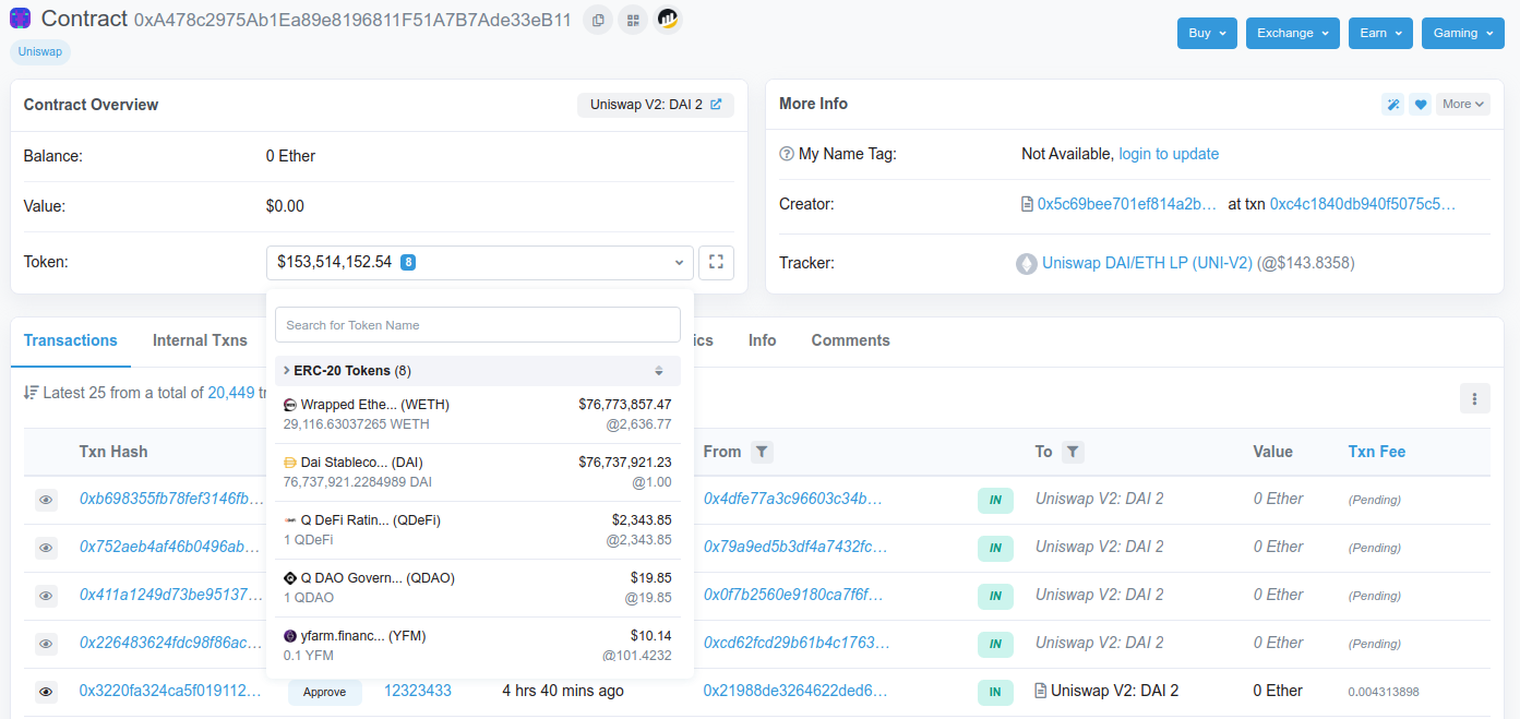
As you can see, the contract, at screenshot time, held about $153.5 million USD — about 29.1 thousand in WETH and about 76.7 million in DAI. So, using the above formula, we can derive k for this pool at this moment in time:

29,116.63 \ast 76,737,921.22 \approx 2.23 * 10^{12}

In any case, unless you are developing apps around Uniswap, k doesn’t really concern you. What you need to know is that it is a number that changes only when someone adds or removes liquidity, or when fees are collected on trades.

In the case of Uniswap, for example, a 0.3% fee is deducted from each trade and added to the total liquidity in the pool. Here’s a more detailed example of an interaction with an AMM-based pool:

1. I stake 1 ETH and 100 DAI in the respective pool on Uniswap
2. With my stake, the total liquidity in the pool becomes 10 ETH and 1,000 DAI — my stake in the pool is 10%
3. Various trades are performed in the pool during a one-week period, amounting to a total volume worth of 100 ETH (50% in ETH and 50% in DAI), but the price of ETH remains the same with regards to DAI
4. No liquidity is added to or removed from the pool in this one-week period
5. The total liquidity in the pool is now 10.15 ETH and 1,015 DAI because of the 0.3 ETH worth of trading fees the pool has collected
6. My stake is still 10%, but it has now grown because of the collected trading fees
7. There is no impermanent loss if I decide to withdraw after that one-week period since the price ratio between ETH and DAI has remained the same

Impermanent Loss in Standard Pools

Let’s use the Uniswap ETH-DAI pool again.

1. I stake 1 ETH and 100 DAI in the pool
2. There’s a total of 10 ETH and 1,000 DAI in the pool after my staking — I have a 10% stake
3. In a week 1 ETH trades for 200 DAI
4. There are no trading fees in the pool

Let’s calculate the impermanent loss from this example. First off, and easiest, we calculate k:

k = 10 * 1,000 = 10,000

Since ETH has doubled in price relative to DAI, arbitrageurs will have used the opportunity to buy cheap ETH from the pool until its price reaches 200 DAI a piece (the overall market price). Remember, at the start of the week we had 10 ETH and 1,000 DAI in the pool, but that was at a price of 100 DAI per ETH. Let’s calculate the new distribution of assets in the pool after the price increase of ETH. To do that, we need to establish a few variables, starting the the price ratio between the assets in the pool:

r_t = a\space price \space in \space b
\\
where
\\
a \space and \space b \space are \space the \space two \space assets \space in \space the \space pool

In our example, a is ETH and b is DAI. Also in our example, 1 ETH traded for 100 DAI at the start. Therefore initial r is 100; we use t to depict the time in which r is calculated. Combining the above equation with the fundamental formula of AMM, we can extract formulae to calculate the amount of each asset in the pool at any given ratio r at any given time t:

\begin{align}x_t = \sqrt{k / r_t}\\
y_t = \sqrt{k*r_t}\end{align}

Let’s apply these formulae to our starting position to see if it works out:

x_{t1} = \sqrt{10,000 / 100} = 10
\\
y_{t1} = \sqrt{10,000 * 100} = 1,000

It works. We get the initial state of the assets in the pool — 10 ETH and 1,000 DAI. Now let’s apply the same formulae for the end of our example, when 1 ETH trades for 200 DAI. Our new r is 200. Let’s plug that into the equations:

x_{t2} = \sqrt{10,000 / 200} \approx 7.07
\\
y_{t2} = \sqrt{10,000 * 200} \approx 1,414.21

After the change in the price of ETH, the pool contains about 7 ETH and about 1,414 DAI. We can confirm that this is correct:

7.07 * 1,414.21 \approx 10,000

Our constant product equation is in tact. Now, we know that our stake in the pool is 10%, so after the price change of ETH, we are entitled to 0.707 ETH and 141.421 DAI. Remember, if we simply held the assets (1 ETH and 100 DAI) we would now have $300 worth of assets.

However, since we are a participant in an AMM-based pool, our worth in USD is:

0.707 * 200 +141.421 = 282.821

Using this, we can calculate the impermanent loss from this example:

300 - 282.821 = 17.179
\\
17.179 / 300 \approx 0.0572 \approx 5.72\%

17.179 DAI, or about 5.72%, is what we would have gained if we simply held the assets instead of staking them in the pool. It is important to note that we have still gained on our initial position of 200 DAI, but in this simple example, the optimal thing would have been to hold the assets.

Here’s a straightforward formula for calculating impermanent loss:

\begin{align}{stake_{USD} \over hold_{USD}} - 1\end{align}

Let’s apply the formula to our example:

{282.821 \over 300} - 1 \approx -0.0572 \approx -5.72\%

Exactly what we were looking for.

To find the exact stake you have in a pool (in each token), either use formulae (2) and (3), or use native analytics platforms such as Uniswap Analytics and SushiSwap Analytics, or third-party tools such as Croco Finance, Growing, and APY.vision.

Accounting For Trading Fees

Note that we excluded trading fees in the previous example. While that makes it easier to calculate impermanent loss, it isn’t the correct way to do it since trading fees are an integral part of AMM-based platforms. Essentially, the more trading fees are collected, the less the impermanent loss; at a critical threshold of trading fees, the impermanent loss becomes positive, meaning you have gained more from participating in the pool compared to holding the assets. Okay, let’s take the above example and add a trading fee component:

1. I stake 1 ETH and 100 DAI in the pool
2. There’s a total of 10 ETH and 1,000 DAI in the pool after my staking — I have a 10% stake
3. In a week 1 ETH trades for 200 DAI
4. This time though, 1 ETH and 100 DAI in trading fees have been collected

We know that, without taking into account trading fees, our impermanent loss here is 17.179 DAI. Since we have a 10% stake in the pool we are entitled to 0.1 ETH and 10 DAI from the accumulated fees. And since ETH is trading at 200 DAI a piece, this 0.1 ETH is worth 20 DAI, making our total gains from fees 30 DAI. This makes our total stake (in USD) 312.821 (282.821 + 30).

Let’s insert these new numbers in formula (4):

{312.821 \over 300} - 1 \approx 0.042 \approx 4.2\%

In this example our impermanent loss is -12.821 DAI (17.179 – 30), which is obviously not a loss, but rather a 4.2% gain — all thanks to our staking in the pool instead of holding.

Plotting Impermanent Loss

So far, we have used the straightforward formula (4) to calculate impermanent loss. While it is great for measuring your current IL, it’s not convenient if you are looking to plot different IL values for different price changes.

From formulae (1), (2), and (3), we can derive another one to easily plot different impermanent loss for different price changes:

2 * {\sqrt{p} \over p + 1} - 1
\\~\\
where
\\
p = r_{t1} / r_{t2}

Let’s apply this formula to our example. We know that initial r is 100 (1 ETH trades for 100 DAI) and final r is 200. Therefore p is 0.5 (100/200). Let’s plug those in:

2 * {\sqrt{0.5} \over 1 + 0.5} - 1 \approx -0.0572 \approx -5.72\%

Exactly the number we got with formula (4). Using this formula, and manipulating for p, allows you to plot different IL at different price changes.

Note that this formula doesn’t account for trading fees. If you’d like to plot for trading fees as well, the formula is this:

2 * {\sqrt{p} \over p + 1} + {fees_{USD} \over hold_{USD}} - 1

You can make estimates of the fees you will collect based on APY data provided by the AMM platform.

Impermanent Loss in Complex Pools

Standard AMM-based pools, such as those on Uniswap and SushiSwap, follow two basic principles:

1. There’s two assets in the pool
2. Each asset composes 50% of the pool

Self-evidently, these pools offer identical exposure to both assets since price changes in either will affect the pool in the same way.

To overcome this limitation, platforms such as Balancer offer pools with different weights and a variable number of assets. For instance, one of the most popular pools on Balancer is BAL-ETH, where the weight of the BAL side of the pool is 80%. This means that changes in the price of ETH (positive or negative) will not affect the pool that much compared to a 50/50 split.

In the case of pools where the weight is not a fifty-fifty, formulae (1), (2), and (3) will not work. So, let’s get k for pools with different weights and a variable number of assets:

k = \displaystyle\prod_i(b_i)^{w_i}
\\~\\
where
\\
b_i \space is \space balance \space of \space token \space i
\\
w_i \space is \space weight \space of \space token \space i

Let’s apply this with a new example; we will use the BAL-ETH pool on Balancer. We have the following:

1. I stake 1 ETH and 10 BAL — ETH trades for $10, BAL trades for $1
2. The total in the pool after my staking is 10 ETH and 100 BAL — my stake is 10%
3. The weight distribution is 80% for BAL and 20% for ETH
4. No liquidity is added or removed in a one-week period
5. In that same period, 1 ETH and 10 BAL in trading fees was collected
6. After this period, the USD price of BAL has doubled (1 ETH trades for 5 BAL) — ETH is $10, BAL is $2

Not that we will need it, but here’s what k is for this example:

k = 10^{0.2}*100^{0.8} \approx 63.0957

Now, for complex pools, the impermanent loss formula is the following:

\begin{align}
{\prod_i(\Delta p_{USD}^i)^{w_i} \over \sum_i(\Delta p_{USD}^i * w_i)} -1 \space
\end{align}
\\~\\
where
\\
w_i \space is \space weight \space of \space token \space i
\\
\Delta p_{USD}^i \space is \space price \space change \space in \space USD \space for \space token \space i

While it may look scary, the formula is actually quite simple: subtract one from the quotient of the product of all token USD price changes in each token to the power of their weight and the sum of all token USD price changes multiplied by their weight. You can find how we get to this formula in this Balancer document.

In our example, we know that ETH’s price hasn’t changed from its initial value of $10, and we know that BAL’s price has doubled from $1 to $2. Therefore, the price change for ETH is 1 (10/10), while the price change for BAL is 2 (2/1). Let’s insert the numbers into the formula:

{1^{0.2} * 2^{0.8} \over 1*0.2 + 2*0.8} - 1 \approx -0.0327 \approx -3.27\%

If you remember, a doubling in the price of one of the assets relative to the other in a standard pool resulted in 5.72% impermanent loss. However, in this case, since the weight of the BAL pool is 80%, we have less impermanent loss.

Formula (5) will work for standard pools as well — you just need to use 0.5 for both weights.

Again, this formula doesn’t account for trading fees. If you want to plot for trading fees as well, the formula is this:

{\prod_i(\Delta p_{USD}^i)^{w_i} \over \sum_i(\Delta p_{USD}^i * w_i)} + {fees_{USD} \over hold_{USD}} -1

Summary

Understanding impermanent loss is necessary for anyone who uses automated market makers because it helps in determining when to open and close positions. Generally speaking, you will always incur some level of impermanent loss when you participate in AMM-based protocols, regardless of price movement. Compared to holding, if asset prices go up, your position will grow less, and if prices go down, you will lose more. This is where trading fees and yield farming come in — they help negate impermanent loss such that your participating in the automated market maker is more profitable than simply holding.